🥇 Tutorial 03: Gold Layer
Last Updated: 2026-04-15 | Version: 2.0 Status: ✅ Final | Maintainer: Documentation Team
🏠 Home > 📖 Tutorials > 🥇 Gold Layer



🥇 Tutorial 03: Gold Layer - Business-Ready Aggregations
| Difficulty | ⭐⭐ Intermediate |
| Time | ⏱️ 60-90 minutes |
| Layer | 🥇 Gold (Business Ready) |
📍 Progress Tracker
| Tutorial | Name | Status | Duration | Difficulty |
|---|---|---|---|---|
| 00 | ⚙️ Environment Setup |  | 45-60 min | ⭐ Beginner |
| 01 | 🥉 Bronze Layer | | 60-90 min | ⭐ Beginner |
| 02 | 🥈 Silver Layer | | 60-90 min | ⭐⭐ Intermediate |
| 03 | 👉 🥇 Gold Layer |  | 90-120 min | ⭐⭐ Intermediate |
| 04 | ⚡ Real-Time Analytics |  | 90-120 min | ⭐⭐⭐ Advanced |
| 05 | 📊 Direct Lake & Power BI | | 60-90 min | ⭐⭐ Intermediate |
| 06 | 🔄 Data Pipelines | | 60-90 min | ⭐⭐ Intermediate |
| 07 | 🛡️ Governance & Purview | | 60-90 min | ⭐⭐ Intermediate |
| 08 | 🔄 Database Mirroring | | 60-90 min | ⭐⭐ Intermediate |
| 09 | 🤖 Advanced AI/ML | | 90-120 min | ⭐⭐⭐ Advanced |
💡 Tip: Click any tutorial name to jump directly to it
| Navigation | |
|---|---|
| ⬅️ Previous | 02-Silver Layer |
| ➡️ Next | 04-Real-Time Analytics |
📖 Overview
This tutorial covers implementing the Gold layer - the crown jewel of the medallion architecture. The Gold layer provides business-ready aggregations, pre-computed KPIs, and star schema structures optimized for analytics and reporting.
Medallion Architecture in Microsoft Fabric
The Gold layer represents the business-ready, aggregated data tier in the medallion lakehouse architecture:
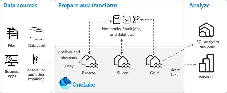
Source: Implement medallion lakehouse architecture in Fabric
flowchart LR
    subgraph Silver["🥈 Silver Layer"]
        S1[Cleansed Slots]
        S2[Player Master]
        S3[Financial Txns]
        S4[Table Games]
    end

    subgraph Gold["🥇 Gold Layer"]
        direction TB
        G1[Slot Performance<br/>Daily KPIs]
        G2[Player 360<br/>Complete View]
        G3[Compliance<br/>Reports]
        G4[Dimensions<br/>Date, Machine]
    end

    subgraph Analytics["📊 Analytics"]
        PBI[Power BI<br/>Direct Lake]
    end

    S1 --> G1
    S2 --> G2
    S3 --> G2
    S4 --> G2
    S3 --> G3

    G1 --> PBI
    G2 --> PBI
    G3 --> PBI
    G4 --> PBI

    style Gold fill:#FFD700,stroke:#B8860B,stroke-width:2px
📊 Visual Overview
The following ERD illustrates the Gold layer star schema design for casino analytics, showing fact tables and their relationships with dimension tables optimized for Power BI Direct Lake mode.
%%{init: {'theme':'base', 'themeVariables': {'primaryColor':'#FFD700','primaryTextColor':'#000','primaryBorderColor':'#B8860B','lineColor':'#4682B4','secondaryColor':'#FFF8DC','tertiaryColor':'#fff'}}}%%
erDiagram
    %% Dimension Tables
    DIM_DATE {
        int date_key PK
        date calendar_date
        int year
        int quarter
        int month
        int day
        string month_name
        string day_name
        int fiscal_year
        int fiscal_quarter
        boolean is_weekend
        boolean is_holiday
    }

    DIM_MACHINE {
        int machine_key PK
        string machine_id UK
        string machine_type
        string manufacturer
        string model
        string denomination
        string floor_section
        int floor_position
        decimal theoretical_hold_pct
        date install_date
        date last_maintenance_date
        string status
    }

    DIM_PLAYER {
        int player_key PK
        string player_id UK
        string tier_status
        date enrollment_date
        date tier_effective_date
        string preferred_game_type
        int lifetime_visits
        decimal lifetime_coin_in
        string risk_category
        string current_status
        date last_visit_date
    }

    DIM_GAME {
        int game_key PK
        string game_id UK
        string game_name
        string game_theme
        string game_category
        string vendor
        decimal min_bet
        decimal max_bet
        string volatility_rating
        decimal rtp_percentage
    }

    DIM_LOCATION {
        int location_key PK
        string floor_section
        string zone_name
        int floor_number
        string casino_area
        int total_machines
        decimal square_footage
    }

    %% Fact Tables
    FACT_SLOT_PERFORMANCE {
        int perf_key PK
        int date_key FK
        int machine_key FK
        int game_key FK
        int location_key FK
        decimal total_coin_in
        decimal total_coin_out
        decimal total_jackpots
        decimal net_win
        decimal theoretical_win
        decimal variance
        int total_spins
        int total_sessions
        decimal avg_bet_amount
        decimal hold_percentage
        decimal player_count
        decimal peak_hour_utilization
    }

    FACT_PLAYER_ACTIVITY {
        int activity_key PK
        int date_key FK
        int player_key FK
        int machine_key FK
        int game_key FK
        timestamp session_start
        timestamp session_end
        int session_duration_min
        decimal total_coin_in
        decimal total_coin_out
        decimal net_win_loss
        int total_spins
        decimal avg_bet
        decimal max_bet
        int jackpot_count
        decimal comp_points_earned
        decimal theo_value
    }

    FACT_FINANCIAL_TXN {
        int txn_key PK
        int date_key FK
        int player_key FK
        string transaction_id UK
        string transaction_type
        decimal amount
        string payment_method
        timestamp transaction_timestamp
        string status
        string location_code
        string processed_by
        boolean compliance_flagged
    }

    FACT_DAILY_KPI {
        int kpi_key PK
        int date_key FK
        int location_key FK
        decimal total_revenue
        decimal total_coin_in
        decimal total_coin_out
        decimal total_jackpots
        decimal hold_percentage
        int active_machines
        int active_players
        int new_enrollments
        decimal avg_session_length
        decimal player_reinvestment_rate
        decimal compliance_score
    }

    %% Relationships - Fact_Slot_Performance
    FACT_SLOT_PERFORMANCE ||--o{ DIM_DATE : "occurs_on"
    FACT_SLOT_PERFORMANCE ||--o{ DIM_MACHINE : "played_on"
    FACT_SLOT_PERFORMANCE ||--o{ DIM_GAME : "features"
    FACT_SLOT_PERFORMANCE ||--o{ DIM_LOCATION : "located_in"

    %% Relationships - Fact_Player_Activity
    FACT_PLAYER_ACTIVITY ||--o{ DIM_DATE : "occurs_on"
    FACT_PLAYER_ACTIVITY ||--o{ DIM_PLAYER : "performed_by"
    FACT_PLAYER_ACTIVITY ||--o{ DIM_MACHINE : "played_on"
    FACT_PLAYER_ACTIVITY ||--o{ DIM_GAME : "features"

    %% Relationships - Fact_Financial_Txn
    FACT_FINANCIAL_TXN ||--o{ DIM_DATE : "occurs_on"
    FACT_FINANCIAL_TXN ||--o{ DIM_PLAYER : "made_by"

    %% Relationships - Fact_Daily_KPI
    FACT_DAILY_KPI ||--o{ DIM_DATE : "summarizes"
    FACT_DAILY_KPI ||--o{ DIM_LOCATION : "for_location"
Star Schema Benefits: - Optimized Queries: Denormalized dimensions for fast aggregations - Direct Lake Ready: Designed for Power BI Direct Lake mode - Business-Aligned: Dimensions match business reporting needs - Pre-Aggregated: Fact tables contain computed KPIs for performance
Key Design Patterns: - Conformed Dimensions: DIM_DATE and DIM_PLAYER shared across all facts - Gaming KPIs: Coin-in, coin-out, hold percentage, theoretical win - Surrogate Keys: Integer keys (_key) for optimal join performance - **SCD Type 2*: Player and Machine dimensions track historical changes - Grain Definition: Daily aggregations in FACT_SLOT_PERFORMANCE, session-level in FACT_PLAYER_ACTIVITY
Casino-Specific Metrics: - Hold Percentage: (Coin-In - Coin-Out) / Coin-In × 100 - Theoretical Win: Expected casino win based on game math - Variance: Actual win vs. theoretical win - Player Reinvestment Rate: Percentage of winnings replayed
🎯 Learning Objectives
By the end of this tutorial, you will be able to:
- Understand Gold layer principles and business alignment
- Create slot machine performance metrics with gaming KPIs
- Build a comprehensive Player 360 view with churn scoring
- Implement compliance reporting tables
- Design star schema with dimension tables
- Optimize for Direct Lake mode in Power BI
🥇 Gold Layer Principles
The Gold layer provides business-ready, aggregated data optimized for consumption:
| Principle | Description | Example |
|---|---|---|
| Business-Aligned | Organized by business domain | Slots, Players, Compliance |
| Aggregated | Pre-computed KPIs and metrics | Daily Theo Win, Hold % |
| Optimized | Designed for query performance | Partitioned, Z-ordered |
| Star Schema | Fact and dimension tables | Fact_SlotPerformance + Dim_Date |
| Direct Lake Ready | Optimized for Power BI | Proper data types, column ordering |
Gaming Industry KPIs
mindmap
  root((Casino KPIs))
    Revenue
      Coin-In
      Coin-Out
      Net Win
      Theo Win
    Performance
      Hold Percentage
      Actual vs Theoretical
      Games Played
    Player
      ADT Average Daily Theo
      Total Visits
      Churn Risk
    Compliance
      CTR Count
      SAR Count
      W2G Amount
📋 Prerequisites
Before starting this tutorial, ensure you have:
- Completed Tutorial 02: Silver Layer
- All Silver tables populated and verified
- Access to
lh_goldLakehouse - Understanding of dimensional modeling concepts
💡 Tip: Run the Silver layer verification notebook before starting to ensure all source tables are ready.
🛠️ Step 1: Slot Performance Metrics
Understanding Gaming KPIs
Before building the Gold table, let's understand key gaming metrics:
| KPI | Formula | Description |
|---|---|---|
| Coin-In | Sum of all wagers | Total money wagered |
| Coin-Out | Sum of all payouts | Total money paid out |
| Net Win | Coin-In - Coin-Out | Casino's actual profit |
| Theo Win | Coin-In × Theoretical Hold % | Expected casino profit |
| Hold % | Net Win / Coin-In × 100 | Actual hold percentage |
| Hold Variance | Actual Hold % - Theoretical Hold % | Performance vs expectation |
Create Notebook: 01_gold_slot_performance
# Cell 1: Configuration
from pyspark.sql import SparkSession
from pyspark.sql.functions import *
from pyspark.sql.types import *
from datetime import datetime

SILVER_TABLE = "lh_silver.silver_slot_cleansed"
GOLD_TABLE = "gold_slot_performance"

print("=" * 60)
print("🥇 GOLD LAYER - Slot Machine Performance Metrics")
print("=" * 60)
print(f"Source: {SILVER_TABLE}")
print(f"Target: {GOLD_TABLE}")
# Cell 2: Read Silver Data
df_silver = spark.table(SILVER_TABLE)

print(f"\n📊 Silver Layer Statistics:")
print(f"  Total Records: {df_silver.count():,}")
print(f"  Date Range: {df_silver.agg(min('event_date'), max('event_date')).first()}")
print(f"  Unique Machines: {df_silver.select('machine_id').distinct().count():,}")
# Cell 3: Calculate Daily Machine Performance Aggregations
print("\n📈 Building Daily Aggregations...")

df_daily = df_silver \
    .filter(col("event_type") == "GAME_PLAY") \
    .groupBy(
        col("machine_id"),
        col("event_date").alias("business_date"),
        col("zone"),
        col("machine_type"),
        col("denomination"),
        col("manufacturer"),
        col("game_theme")
    ) \
    .agg(
        # Volume Metrics
        count("*").alias("total_games"),
        countDistinct("player_id").alias("unique_players"),
        countDistinct("session_id").alias("total_sessions"),

        # Financial Metrics (in cents, will convert to dollars)
        sum("coin_in").alias("total_coin_in"),
        sum("coin_out").alias("total_coin_out"),
        sum("jackpot_amount").alias("total_jackpots"),

        # Performance Metrics
        avg("coin_in").alias("avg_bet"),
        max("coin_in").alias("max_bet"),
        avg("theoretical_hold").alias("avg_theoretical_hold"),

        # Time Metrics
        min("event_timestamp").alias("first_play"),
        max("event_timestamp").alias("last_play")
    )

print(f"  Daily aggregations created: {df_daily.count():,} rows")
KPI Calculations
# Cell 4: Calculate Gaming KPIs
print("\n🎰 Calculating Gaming KPIs...")

df_kpis = df_daily \
    .withColumn("net_win",
        col("total_coin_in") - col("total_coin_out")) \
    .withColumn("actual_hold_pct",
        when(col("total_coin_in") > 0,
             round((col("total_coin_in") - col("total_coin_out")) / col("total_coin_in") * 100, 2))
        .otherwise(0)) \
    .withColumn("theo_win",
        round(col("total_coin_in") * col("avg_theoretical_hold"), 2)) \
    .withColumn("hold_variance",
        round(col("actual_hold_pct") - (col("avg_theoretical_hold") * 100), 2)) \
    .withColumn("hold_performance",
        when(col("hold_variance") > 2, "OVER_PERFORMING")
        .when(col("hold_variance") < -2, "UNDER_PERFORMING")
        .otherwise("ON_TARGET")) \
    .withColumn("avg_session_length_games",
        when(col("total_sessions") > 0,
             round(col("total_games") / col("total_sessions"), 1))
        .otherwise(0)) \
    .withColumn("games_per_player",
        when(col("unique_players") > 0,
             round(col("total_games") / col("unique_players"), 1))
        .otherwise(0)) \
    .withColumn("jackpot_hit_rate",
        when(col("total_games") > 0,
             round(col("total_jackpots") / col("total_games"), 4))
        .otherwise(0)) \
    .withColumn("revenue_per_player",
        when(col("unique_players") > 0,
             round(col("net_win") / col("unique_players"), 2))
        .otherwise(0))

print("  KPIs calculated:")
print("    - net_win, actual_hold_pct, theo_win")
print("    - hold_variance, hold_performance")
print("    - avg_session_length_games, games_per_player")
print("    - jackpot_hit_rate, revenue_per_player")
💡 Tip: Hold variance is a critical metric for slot operations. Machines consistently outside the -2% to +2% range may need investigation.
# Cell 5: Add Gold Metadata and Finalize Schema
print("\n✨ Finalizing Gold Table Schema...")

df_gold = df_kpis \
    .withColumn("_gold_processed_at", current_timestamp()) \
    .withColumn("_gold_batch_id", lit(datetime.now().strftime("%Y%m%d")))

# Reorder columns for clarity and Direct Lake optimization
column_order = [
    # Keys (frequently filtered - put first for Direct Lake)
    "business_date", "machine_id", "zone", "machine_type", "denomination",
    "manufacturer", "game_theme",

    # Volume Metrics
    "total_games", "unique_players", "total_sessions",

    # Financial Metrics
    "total_coin_in", "total_coin_out", "net_win", "total_jackpots",

    # Performance KPIs
    "actual_hold_pct", "avg_theoretical_hold", "theo_win", "hold_variance",
    "hold_performance",

    # Player Metrics
    "avg_bet", "max_bet", "avg_session_length_games", "games_per_player",
    "jackpot_hit_rate", "revenue_per_player",

    # Time
    "first_play", "last_play",

    # Metadata
    "_gold_processed_at", "_gold_batch_id"
]

df_gold = df_gold.select(column_order)
# Cell 6: Write to Gold Table with Optimization
print("\n💾 Writing to Gold Table...")

df_gold.write \
    .format("delta") \
    .mode("overwrite") \
    .partitionBy("business_date") \
    .saveAsTable(GOLD_TABLE)

# Optimize for query performance
spark.sql(f"OPTIMIZE {GOLD_TABLE} ZORDER BY (machine_id, zone)")

print(f"✅ Wrote {df_gold.count():,} records to {GOLD_TABLE}")
print("✅ Applied Z-ORDER optimization on (machine_id, zone)")
# Cell 7: Verify and Analyze
df_verify = spark.table(GOLD_TABLE)

print("\n" + "=" * 60)
print("✅ SLOT PERFORMANCE VERIFICATION")
print("=" * 60)

print(f"\n📊 Gold Table Statistics:")
print(f"  Total Records: {df_verify.count():,}")
date_range = df_verify.agg(min('business_date'), max('business_date')).first()
print(f"  Date Range: {date_range[0]} to {date_range[1]}")

print("\n🏆 Top 10 Machines by Net Win:")
display(
    df_verify
    .groupBy("machine_id", "machine_type", "zone")
    .agg(
        sum("net_win").alias("total_net_win"),
        avg("actual_hold_pct").alias("avg_hold_pct"),
        sum("total_games").alias("total_games")
    )
    .orderBy(col("total_net_win").desc())
    .limit(10)
)

print("\n📉 Machines with Hold Variance Issues:")
display(
    df_verify
    .filter(abs(col("hold_variance")) > 3)
    .groupBy("machine_id", "zone", "hold_performance")
    .agg(
        avg("hold_variance").alias("avg_variance"),
        count("*").alias("days_with_variance")
    )
    .orderBy(col("days_with_variance").desc())
    .limit(10)
)
🛠️ Step 2: Player 360 View
Understanding Player 360
The Player 360 view combines data from multiple sources to create a complete picture of each player:
flowchart TB
    subgraph Sources["Data Sources"]
        PM[Player Master<br/>Demographics, Tier]
        SLOT[Slot Activity<br/>Games, Coin-in]
        TBL[Table Activity<br/>Wagered, Win/Loss]
        FIN[Financial<br/>Cash-in, Cash-out]
    end

    subgraph P360["Player 360 View"]
        PROFILE[Profile Data]
        GAMING[Gaming Summary]
        VALUE[Value Scores]
        RISK[Risk Indicators]
    end

    PM --> PROFILE
    SLOT --> GAMING
    TBL --> GAMING
    FIN --> VALUE
    GAMING --> VALUE
    VALUE --> RISK
Create Notebook: 02_gold_player_360
# Cell 1: Configuration
from pyspark.sql import SparkSession
from pyspark.sql.functions import *
from datetime import datetime

SILVER_PLAYER = "lh_silver.silver_player_master"
SILVER_SLOTS = "lh_silver.silver_slot_cleansed"
SILVER_TABLES = "lh_silver.silver_table_enriched"
SILVER_FINANCIAL = "lh_silver.silver_financial_reconciled"
GOLD_TABLE = "gold_player_360"

print("=" * 60)
print("🥇 GOLD LAYER - Player 360 View")
print("=" * 60)
# Cell 2: Get Current Player Profile Data
print("\n👤 Loading Player Profile Data...")

df_player = spark.table(SILVER_PLAYER) \
    .filter(col("_is_current") == True) \
    .select(
        "player_id", "loyalty_number", "loyalty_tier",
        "enrollment_date", "total_visits", "total_theo",
        "preferred_game", "vip_flag", "self_excluded", "account_status",
        "date_of_birth", "city", "state"
    )

# Calculate age
df_player = df_player.withColumn("age",
    floor(datediff(current_date(), col("date_of_birth")) / 365.25))

print(f"  Active Players: {df_player.count():,}")
print(f"  VIP Players: {df_player.filter(col('vip_flag')).count():,}")
# Cell 3: Calculate Slot Gaming Activity
print("\n🎰 Aggregating Slot Activity...")

df_slot_activity = spark.table(SILVER_SLOTS) \
    .filter(col("player_id").isNotNull()) \
    .filter(col("event_type") == "GAME_PLAY") \
    .groupBy("player_id") \
    .agg(
        count("*").alias("slot_games_played"),
        sum("coin_in").alias("slot_coin_in"),
        sum("coin_out").alias("slot_coin_out"),
        countDistinct("machine_id").alias("unique_machines"),
        countDistinct("event_date").alias("slot_visit_days"),
        max("event_timestamp").alias("last_slot_play"),
        avg("coin_in").alias("avg_slot_bet"),
        max("coin_in").alias("max_slot_bet"),
        # Favorite denomination
        mode("denomination").alias("preferred_denomination")
    )

print(f"  Players with slot activity: {df_slot_activity.count():,}")
# Cell 4: Calculate Table Gaming Activity
print("\n🃏 Aggregating Table Activity...")

df_table_activity = spark.table(SILVER_TABLES) \
    .filter(col("player_id").isNotNull()) \
    .groupBy("player_id") \
    .agg(
        sum("average_bet").alias("table_total_wagered"),
        sum("theoretical_win").alias("table_theo_win"),
        sum("actual_win_loss").alias("table_actual_wl"),
        sum("hours_played").alias("table_hours_played"),
        countDistinct("event_date").alias("table_visit_days"),
        max("event_timestamp").alias("last_table_play"),
        avg("average_bet").alias("avg_table_bet"),
        mode("game_type").alias("preferred_table_game")
    )

print(f"  Players with table activity: {df_table_activity.count():,}")
# Cell 5: Calculate Financial Activity
print("\n💰 Aggregating Financial Activity...")

df_financial = spark.table(SILVER_FINANCIAL) \
    .filter(col("player_id").isNotNull()) \
    .groupBy("player_id") \
    .agg(
        sum(when(col("transaction_type") == "CASH_IN", col("amount"))).alias("total_cash_in"),
        sum(when(col("transaction_type") == "CASH_OUT", col("amount"))).alias("total_cash_out"),
        sum(when(col("transaction_type") == "MARKER_ISSUE", col("amount"))).alias("total_markers_issued"),
        sum(when(col("transaction_type") == "MARKER_PAYMENT", col("amount"))).alias("total_markers_paid"),
        count("*").alias("total_transactions"),
        countDistinct("transaction_date").alias("financial_visit_days")
    )

print(f"  Players with financial activity: {df_financial.count():,}")
# Cell 6: Join All Sources
print("\n🔗 Creating Unified Player View...")

df_360 = df_player \
    .join(df_slot_activity, "player_id", "left") \
    .join(df_table_activity, "player_id", "left") \
    .join(df_financial, "player_id", "left")

# Fill nulls for numeric columns
numeric_cols = [
    "slot_games_played", "slot_coin_in", "slot_coin_out", "unique_machines",
    "slot_visit_days", "avg_slot_bet", "max_slot_bet",
    "table_total_wagered", "table_theo_win", "table_actual_wl", "table_hours_played",
    "table_visit_days", "avg_table_bet",
    "total_cash_in", "total_cash_out", "total_markers_issued", "total_markers_paid",
    "total_transactions", "financial_visit_days"
]
df_360 = df_360.fillna(0, subset=numeric_cols)

print(f"  Combined Player Records: {df_360.count():,}")
Player Value and Risk Scoring
# Cell 7: Calculate Player KPIs and Scores
print("\n📊 Calculating Player KPIs...")

df_gold = df_360 \
    .withColumn("total_gaming_activity",
        col("slot_coin_in") + col("table_total_wagered")) \
    .withColumn("slot_theo_win",
        col("slot_coin_in") * 0.08) \
    .withColumn("total_theo_win",
        col("slot_theo_win") + coalesce(col("table_theo_win"), lit(0))) \
    .withColumn("slot_net_win",
        col("slot_coin_in") - col("slot_coin_out")) \
    .withColumn("total_net_win",
        col("slot_net_win") + coalesce(col("table_actual_wl"), lit(0))) \
    .withColumn("net_cash_position",
        coalesce(col("total_cash_in"), lit(0)) - coalesce(col("total_cash_out"), lit(0))) \
    .withColumn("outstanding_markers",
        coalesce(col("total_markers_issued"), lit(0)) - coalesce(col("total_markers_paid"), lit(0))) \
    .withColumn("last_activity_date",
        greatest(col("last_slot_play"), col("last_table_play"))) \
    .withColumn("days_since_visit",
        datediff(current_date(), col("last_activity_date"))) \
    .withColumn("total_visit_days",
        col("slot_visit_days") + col("table_visit_days"))
# Cell 8: Calculate Risk and Value Indicators
print("\n⚠️ Calculating Risk Indicators...")

df_gold = df_gold \
    .withColumn("churn_risk",
        when(col("days_since_visit") > 90, "HIGH")
        .when(col("days_since_visit") > 60, "MEDIUM_HIGH")
        .when(col("days_since_visit") > 30, "MEDIUM")
        .when(col("days_since_visit") > 14, "LOW")
        .otherwise("ACTIVE")) \
    .withColumn("player_value_tier",
        when(col("total_theo_win") >= 10000, "WHALE")
        .when(col("total_theo_win") >= 5000, "HIGH_VALUE")
        .when(col("total_theo_win") >= 1000, "MEDIUM_VALUE")
        .when(col("total_theo_win") >= 100, "LOW_VALUE")
        .otherwise("MINIMAL")) \
    .withColumn("player_value_score",
        # Composite score: Theo Win + Visit Frequency + Loyalty Tier bonus
        (col("total_theo_win") / 100) +
        (col("total_visit_days") * 10) +
        when(col("loyalty_tier") == "Diamond", 500)
        .when(col("loyalty_tier") == "Platinum", 200)
        .when(col("loyalty_tier") == "Gold", 100)
        .when(col("loyalty_tier") == "Silver", 50)
        .otherwise(10)) \
    .withColumn("engagement_score",
        # Based on recency and frequency
        when(col("days_since_visit") <= 7, 100)
        .when(col("days_since_visit") <= 14, 80)
        .when(col("days_since_visit") <= 30, 60)
        .when(col("days_since_visit") <= 60, 40)
        .when(col("days_since_visit") <= 90, 20)
        .otherwise(0) +
        least(col("total_visit_days"), lit(100))) \
    .withColumn("credit_risk",
        when(col("outstanding_markers") > 10000, "HIGH")
        .when(col("outstanding_markers") > 5000, "MEDIUM")
        .when(col("outstanding_markers") > 0, "LOW")
        .otherwise("NONE")) \
    .withColumn("_gold_processed_at", current_timestamp())
⚠️ Warning: Player value scores and risk indicators should be reviewed by marketing and compliance teams before use in campaigns.
# Cell 9: Write Player 360 Gold Table
print("\n💾 Writing Player 360 Gold Table...")

df_gold.write \
    .format("delta") \
    .mode("overwrite") \
    .saveAsTable(GOLD_TABLE)

# No partitioning for dimension-like table, but optimize
spark.sql(f"OPTIMIZE {GOLD_TABLE} ZORDER BY (loyalty_tier, churn_risk)")

print(f"✅ Wrote {df_gold.count():,} player 360 records")
# Cell 10: Verify and Analyze
print("\n" + "=" * 60)
print("✅ PLAYER 360 VERIFICATION")
print("=" * 60)

df_verify = spark.table(GOLD_TABLE)

print("\n📊 Player Distribution by Value Tier:")
display(
    df_verify
    .groupBy("player_value_tier")
    .agg(
        count("*").alias("player_count"),
        round(avg("total_theo_win"), 2).alias("avg_theo_win"),
        round(avg("total_visit_days"), 1).alias("avg_visits")
    )
    .orderBy(col("avg_theo_win").desc())
)

print("\n⚠️ Churn Risk Analysis:")
display(
    df_verify
    .groupBy("churn_risk", "loyalty_tier")
    .agg(
        count("*").alias("player_count"),
        round(sum("total_theo_win"), 2).alias("total_theo_at_risk")
    )
    .orderBy("churn_risk", col("total_theo_at_risk").desc())
)

print("\n🏆 Top 20 Players by Value Score:")
display(
    df_verify
    .select(
        "player_id", "loyalty_tier", "player_value_tier",
        "total_theo_win", "total_visit_days", "churn_risk",
        "player_value_score", "engagement_score"
    )
    .orderBy(col("player_value_score").desc())
    .limit(20)
)
🛠️ Step 3: Compliance Reporting
Create Notebook: 03_gold_compliance_reporting
# Cell 1: Configuration
from pyspark.sql import SparkSession
from pyspark.sql.functions import *
from datetime import datetime

SILVER_TABLE = "lh_silver.silver_compliance_validated"
GOLD_TABLE = "gold_compliance_reporting"

print("=" * 60)
print("🥇 GOLD LAYER - Compliance Reporting")
print("=" * 60)
# Cell 2: Read and Aggregate Daily Compliance Summary
df_silver = spark.table(SILVER_TABLE)

print("\n📋 Building Daily Compliance Summary...")

df_daily = df_silver \
    .withColumn("report_date", to_date(col("filing_date"))) \
    .groupBy("report_date", "report_type", "status") \
    .agg(
        count("*").alias("report_count"),
        sum("transaction_amount").alias("total_amount"),
        avg("transaction_amount").alias("avg_amount"),
        countDistinct("player_id").alias("unique_patrons"),
        countDistinct("transaction_id").alias("unique_transactions")
    )

print(f"  Daily summaries: {df_daily.count():,}")
# Cell 3: Pivot by Report Type for Dashboard View
print("\n📊 Creating Pivoted Report View...")

df_pivot = df_silver \
    .withColumn("report_date", to_date(col("filing_date"))) \
    .groupBy("report_date") \
    .pivot("report_type", ["CTR", "SAR", "W2G", "MTLAP", "CTRC"]) \
    .agg(
        count("*").alias("count"),
        sum("transaction_amount").alias("amount")
    )

# Clean up column names
for col_name in df_pivot.columns:
    if col_name != "report_date":
        new_name = col_name.lower().replace(" ", "_")
        df_pivot = df_pivot.withColumnRenamed(col_name, new_name)

df_pivot = df_pivot.fillna(0)
# Cell 4: Add Compliance KPIs and Alert Levels
print("\n⚠️ Calculating Compliance KPIs...")

df_gold = df_pivot \
    .withColumn("total_filings",
        coalesce(col("ctr_count"), lit(0)) +
        coalesce(col("sar_count"), lit(0)) +
        coalesce(col("w2g_count"), lit(0)) +
        coalesce(col("mtlap_count"), lit(0)) +
        coalesce(col("ctrc_count"), lit(0))) \
    .withColumn("total_reportable_amount",
        coalesce(col("ctr_amount"), lit(0)) +
        coalesce(col("sar_amount"), lit(0)) +
        coalesce(col("w2g_amount"), lit(0))) \
    .withColumn("ctr_compliance_status",
        when(col("ctr_count") > 0, "FILINGS_PRESENT")
        .otherwise("NO_FILINGS")) \
    .withColumn("sar_alert_level",
        when(col("sar_count") > 10, "CRITICAL")
        .when(col("sar_count") > 5, "HIGH")
        .when(col("sar_count") > 2, "ELEVATED")
        .when(col("sar_count") > 0, "NORMAL")
        .otherwise("NONE")) \
    .withColumn("w2g_jackpot_activity",
        when(col("w2g_amount") > 100000, "VERY_HIGH")
        .when(col("w2g_amount") > 50000, "HIGH")
        .when(col("w2g_amount") > 10000, "MODERATE")
        .otherwise("NORMAL")) \
    .withColumn("daily_compliance_score",
        # Higher score = better compliance posture
        100 -
        (when(col("sar_alert_level") == "CRITICAL", 30)
         .when(col("sar_alert_level") == "HIGH", 20)
         .when(col("sar_alert_level") == "ELEVATED", 10)
         .otherwise(0))) \
    .withColumn("_gold_processed_at", current_timestamp())
⚠️ Warning: SAR (Suspicious Activity Report) counts at "CRITICAL" level require immediate review by the compliance department.
# Cell 5: Write Compliance Gold Table
print("\n💾 Writing Compliance Reporting Gold Table...")

df_gold.write \
    .format("delta") \
    .mode("overwrite") \
    .partitionBy("report_date") \
    .saveAsTable(GOLD_TABLE)

print(f"✅ Wrote {df_gold.count():,} compliance summary records")
# Cell 6: Verification
print("\n" + "=" * 60)
print("✅ COMPLIANCE REPORTING VERIFICATION")
print("=" * 60)

df_verify = spark.table(GOLD_TABLE)

print("\n📊 Filing Summary by Type:")
display(
    df_verify
    .agg(
        sum("ctr_count").alias("total_ctr"),
        sum("sar_count").alias("total_sar"),
        sum("w2g_count").alias("total_w2g"),
        round(sum("ctr_amount"), 2).alias("ctr_amount"),
        round(sum("w2g_amount"), 2).alias("w2g_amount")
    )
)

print("\n⚠️ Days with Elevated SAR Activity:")
display(
    df_verify
    .filter(col("sar_alert_level").isin(["CRITICAL", "HIGH", "ELEVATED"]))
    .select("report_date", "sar_count", "sar_alert_level", "daily_compliance_score")
    .orderBy(col("sar_count").desc())
    .limit(10)
)
🛠️ Step 4: Create Dimension Tables
Star Schema Design
A proper star schema requires dimension tables for efficient filtering and slicing:
erDiagram
    FACT_SLOT_PERFORMANCE ||--o{ DIM_DATE : business_date
    FACT_SLOT_PERFORMANCE ||--o{ DIM_MACHINE : machine_id
    FACT_SLOT_PERFORMANCE ||--o{ DIM_ZONE : zone_id
    GOLD_PLAYER_360 ||--o{ DIM_DATE : enrollment_date
    GOLD_COMPLIANCE ||--o{ DIM_DATE : report_date

    DIM_DATE {
        date date_key PK
        int year
        int quarter
        int month
        string month_name
        int week
        int day_of_week
        string day_name
        boolean is_weekend
        boolean is_holiday
        int fiscal_year
        int fiscal_quarter
    }

    DIM_MACHINE {
        string machine_id PK
        string asset_number
        string zone
        string machine_type
        string manufacturer
        decimal denomination
        string game_theme
    }

    FACT_SLOT_PERFORMANCE {
        date business_date FK
        string machine_id FK
        int total_games
        decimal coin_in
        decimal net_win
    }
Date Dimension
📦 Shortcut — use the packaged notebook. Both
dim_dateanddim_machineare packaged in notebooks/gold/00_gold_dim_tables.py. Import that single notebook into your Fabric workspace and run it once; it creates both dimensions inlh_gold.dbo.dim_dateandlh_gold.dbo.dim_machine. The code blocks below explain what the notebook does — you do not need to copy-paste them if you imported the notebook.
# Create Date Dimension
from pyspark.sql.functions import *

print("📅 Creating Date Dimension...")

# Generate date range (2 years of history + 1 year future)
start_date = "2023-01-01"
end_date = "2026-12-31"

df_dates = spark.sql(f"""
    SELECT explode(sequence(to_date('{start_date}'), to_date('{end_date}'))) as date_key
""")

df_dim_date = df_dates \
    .withColumn("year", year("date_key")) \
    .withColumn("quarter", quarter("date_key")) \
    .withColumn("month", month("date_key")) \
    .withColumn("month_name", date_format("date_key", "MMMM")) \
    .withColumn("month_abbr", date_format("date_key", "MMM")) \
    .withColumn("week", weekofyear("date_key")) \
    .withColumn("day_of_month", dayofmonth("date_key")) \
    .withColumn("day_of_week", dayofweek("date_key")) \
    .withColumn("day_name", date_format("date_key", "EEEE")) \
    .withColumn("day_abbr", date_format("date_key", "EEE")) \
    .withColumn("is_weekend", dayofweek("date_key").isin([1, 7])) \
    .withColumn("is_weekday", ~dayofweek("date_key").isin([1, 7])) \
    .withColumn("year_month", date_format("date_key", "yyyy-MM")) \
    .withColumn("year_quarter", concat(year("date_key"), lit("-Q"), quarter("date_key"))) \
    .withColumn("fiscal_year",
        when(month("date_key") >= 10, year("date_key") + 1)
        .otherwise(year("date_key"))) \
    .withColumn("fiscal_quarter",
        when(quarter("date_key") >= 4, quarter("date_key") - 3)
        .otherwise(quarter("date_key") + 1)) \
    .withColumn("fiscal_month",
        when(month("date_key") >= 10, month("date_key") - 9)
        .otherwise(month("date_key") + 3))

df_dim_date.write.format("delta").mode("overwrite").saveAsTable("dim_date")
print(f"✅ Created dim_date with {df_dim_date.count():,} dates")
Machine Dimension
# Create Machine Dimension
print("🎰 Creating Machine Dimension...")

df_dim_machine = spark.table("lh_silver.silver_slot_cleansed") \
    .select(
        "machine_id", "asset_number", "location_id", "zone",
        "machine_type", "manufacturer", "game_theme", "denomination",
        "par_percentage", "max_bet", "progressive_flag"
    ) \
    .distinct() \
    .withColumn("machine_key", monotonically_increasing_id()) \
    .withColumn("denomination_display",
        concat(lit("$"), format_number(col("denomination"), 2))) \
    .withColumn("machine_category",
        when(col("machine_type").contains("VIDEO"), "Video")
        .when(col("machine_type").contains("REEL"), "Reel")
        .when(col("progressive_flag"), "Progressive")
        .otherwise("Standard"))

df_dim_machine.write.format("delta").mode("overwrite").saveAsTable("dim_machine")
print(f"✅ Created dim_machine with {df_dim_machine.count():,} machines")
Zone Dimension
# Create Zone Dimension
print("📍 Creating Zone Dimension...")

df_dim_zone = spark.table("lh_silver.silver_slot_cleansed") \
    .select("zone", "location_id") \
    .distinct() \
    .withColumn("zone_key", monotonically_increasing_id()) \
    .withColumn("zone_type",
        when(col("zone").contains("VIP"), "VIP")
        .when(col("zone").contains("HIGH"), "High Limit")
        .when(col("zone").contains("SMOKE"), "Smoking")
        .otherwise("General")) \
    .withColumn("floor_level",
        when(col("zone").contains("LEVEL_1"), 1)
        .when(col("zone").contains("LEVEL_2"), 2)
        .when(col("zone").contains("LEVEL_3"), 3)
        .otherwise(1))

df_dim_zone.write.format("delta").mode("overwrite").saveAsTable("dim_zone")
print(f"✅ Created dim_zone with {df_dim_zone.count():,} zones")
🛠️ Step 5: Gold Layer Verification
# Gold Layer Complete Verification
from pyspark.sql.functions import *
from datetime import datetime

# All Gold tables
gold_tables = [
    ("gold_slot_performance", "Fact"),
    ("gold_player_360", "Aggregate"),
    ("gold_compliance_reporting", "Aggregate"),
    ("gold_table_analytics", "Fact"),
    ("gold_financial_summary", "Aggregate"),
    ("dim_date", "Dimension"),
    ("dim_machine", "Dimension"),
    ("dim_zone", "Dimension")
]

print("=" * 70)
print("🥇 GOLD LAYER VERIFICATION REPORT")
print("=" * 70)
print(f"Timestamp: {datetime.now().strftime('%Y-%m-%d %H:%M:%S')}")
print("-" * 70)

total_records = 0
passed = 0
failed = 0

for table, table_type in gold_tables:
    try:
        df = spark.table(table)
        count = df.count()
        total_records += count

        # Check for Gold metadata
        has_gold_meta = "_gold_processed_at" in df.columns or table.startswith("dim_")
        status = "✅" if has_gold_meta else "⚠️"
        passed += 1

        print(f"{status} [{table_type:10}] {table:30} {count:>12,} records")

    except Exception as e:
        print(f"❌ [{table_type:10}] {table:30} NOT FOUND")
        failed += 1

print("-" * 70)
print(f"{'SUMMARY':45} {total_records:>12,} total records")
print(f"{'Tables Passed:':45} {passed}/{len(gold_tables)}")
if failed > 0:
    print(f"{'Tables Failed:':45} {failed}/{len(gold_tables)}")
print("=" * 70)
⚡ Direct Lake Optimization
Direct Lake mode connects Power BI directly to Delta tables in OneLake for the best of both import and DirectQuery modes:
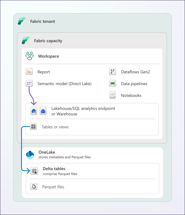
Source: Direct Lake overview
For optimal Power BI Direct Lake performance, follow these guidelines:
1. Column Ordering
Place frequently filtered columns first in the table schema:
# Good: Keys and filter columns first
df.select(
    "business_date",    # Primary filter
    "machine_id",       # Common filter
    "zone",             # Common filter
    "total_coin_in",    # Measure
    "net_win",          # Measure
    ...
)
2. Data Types
Use appropriate types that Direct Lake handles efficiently:
df = df \
    .withColumn("amount", col("amount").cast("decimal(18,2)")) \
    .withColumn("percentage", col("percentage").cast("decimal(5,2)")) \
    .withColumn("is_active", col("is_active").cast("boolean")) \
    .withColumn("count", col("count").cast("integer"))
3. Partitioning Strategy
Partition fact tables by date for time-series queries:
# Fact tables: Partition by date
df.write \
    .partitionBy("business_date") \
    .saveAsTable("gold_slot_performance")

# Dimension tables: No partitioning (small, frequently joined)
df.write \
    .saveAsTable("dim_machine")
4. Table Optimization
Run optimization after writes:
# Z-ORDER by commonly filtered columns
spark.sql(f"OPTIMIZE gold_slot_performance ZORDER BY (machine_id, zone)")

# VACUUM to remove old files (retain 7 days for time travel)
spark.sql(f"VACUUM gold_slot_performance RETAIN 168 HOURS")
5. V-Order (Fabric-Specific)
Enable V-Order for maximum Direct Lake performance:
# V-Order is automatically applied in Fabric
# Verify with:
spark.sql("DESCRIBE DETAIL gold_slot_performance").show()
✅ Validation Checklist
Before moving to the next tutorial, verify:
- All Gold Tables Created - Fact and dimension tables exist in
lh_gold - Star Schema Correct - Relationships between facts and dimensions verified
- Aggregations Work - KPIs calculating correctly (hold %, theo win, etc.)
- Dimension Tables Populated - Date, machine, zone dimensions complete
- Partitioning Applied - Date-based partitions on fact tables
- Optimization Complete - Z-ORDER and VACUUM executed successfully
🔍 How to verify each item
### All Gold Tables Created# List all Gold tables
tables = spark.sql("SHOW TABLES IN lh_gold").collect()
table_names = [row.tableName for row in tables]
expected_tables = [
"gold_slot_performance",
"gold_player_360",
"gold_compliance_reporting",
"dim_date",
"dim_machine",
"dim_zone"
]
for table in expected_tables:
status = "✅" if table in table_names else "❌"
count = spark.table(f"lh_gold.{table}").count() if table in table_names else 0
print(f"{status} {table:30} {count:>10,} rows")
-- Verify fact table can join to all dimensions
SELECT
    f.business_date,
    d.date_name,
    m.machine_name,
    z.zone_name,
    f.total_coin_in,
    f.net_win
FROM lh_gold.gold_slot_performance f
JOIN lh_gold.dim_date d ON f.business_date = d.date_key
JOIN lh_gold.dim_machine m ON f.machine_id = m.machine_id
JOIN lh_gold.dim_zone z ON m.zone_id = z.zone_id
LIMIT 10;

-- Should return results without errors
# Verify KPI calculations
df = spark.table("lh_gold.gold_slot_performance")

# Check hold percentage calculation
df.select(
    "machine_id",
    "business_date",
    "total_coin_in",
    "total_coin_out",
    "net_win",
    "actual_hold_pct",
    ((col("total_coin_in") - col("total_coin_out")) / col("total_coin_in") * 100).alias("calculated_hold_pct")
).show(5)

# Verify actual_hold_pct matches calculated_hold_pct
# Check date dimension coverage
df_date = spark.table("lh_gold.dim_date")
print(f"Date dimension rows: {df_date.count():,}")
print(f"Date range: {df_date.agg({'date_key': 'min'}).collect()[0][0]} to {df_date.agg({'date_key': 'max'}).collect()[0][0]}")

# Check machine dimension
df_machine = spark.table("lh_gold.dim_machine")
print(f"\nMachine dimension rows: {df_machine.count():,}")
df_machine.groupBy("zone_id").count().show()

# Check zone dimension
df_zone = spark.table("lh_gold.dim_zone")
print(f"\nZone dimension rows: {df_zone.count():,}")
df_zone.show()
# Check if tables are partitioned
from delta.tables import DeltaTable

table_name = "lh_gold.gold_slot_performance"
delta_table = DeltaTable.forName(spark, table_name)

# Get table details
details = delta_table.detail().select("partitionColumns").collect()[0]
print(f"Partition columns: {details['partitionColumns']}")

# Should show ['business_date'] or similar date partition
# Check when tables were last optimized
from delta.tables import DeltaTable

table_name = "lh_gold.gold_slot_performance"
delta_table = DeltaTable.forName(spark, table_name)

# Check history for OPTIMIZE operations
history = delta_table.history(10)
optimize_ops = history.filter(col("operation") == "OPTIMIZE")

print("Recent optimization history:")
optimize_ops.select("timestamp", "operation", "operationMetrics").show(truncate=False)

# Also check for VACUUM operations
vacuum_ops = history.filter(col("operation") == "VACUUM END")
print("\nRecent vacuum history:")
vacuum_ops.select("timestamp", "operation", "operationMetrics").show(truncate=False)
-- Verify key metrics are calculating correctly
SELECT
    business_date,
    COUNT(DISTINCT machine_id) as machine_count,
    SUM(total_coin_in) as total_coin_in,
    SUM(total_coin_out) as total_coin_out,
    SUM(net_win) as net_win,
    AVG(actual_hold_pct) as avg_hold_pct,
    SUM(theoretical_win) as total_theo
FROM lh_gold.gold_slot_performance
WHERE business_date >= DATEADD(day, -7, GETDATE())
GROUP BY business_date
ORDER BY business_date DESC;

-- Metrics should be positive and hold % between 5-15%
🎉 Summary
Congratulations! You have successfully implemented the Gold layer:
| Achievement | Description |
|---|---|
| ✅ Slot Performance | Created daily machine KPIs with gaming-specific metrics |
| ✅ Player 360 | Built comprehensive player view with value and risk scoring |
| ✅ Compliance Reporting | Implemented regulatory reporting summaries |
| ✅ Star Schema | Created dimension tables for efficient analytics |
| ✅ Direct Lake Ready | Optimized tables for Power BI consumption |
➡️ Next Steps
Continue to Tutorial 04: Real-Time Analytics to learn:
- Implementing Eventstream for real-time data ingestion
- Building KQL queries for streaming analytics
- Creating real-time dashboards
- Alerting on anomalies
📚 Resources
| Resource | Description |
|---|---|
| Gold Layer Best Practices | Microsoft Fabric medallion patterns |
| Direct Lake Mode | Power BI Direct Lake optimization |
| Star Schema Design | Dimensional modeling guidance |
| Delta Lake Optimization | OPTIMIZE and Z-ORDER |
| Gaming Analytics KPIs | Industry standard metrics |
🧭 Navigation
| ⬅️ Previous | ⬆️ Up | ➡️ Next |
|---|---|---|
| 02-Silver Layer | Tutorials Index | 04-Real-Time Analytics |
Questions or issues? Open an issue in the GitHub repository.
🥇 Gold Layer - Business-ready insights at your fingertips