
⚡ Performance Optimization Best Practices
Home > Best Practices > Performance Optimization
🚀 Performance Excellence Framework
Comprehensive guide to optimizing performance across all Azure Synapse Analytics components for maximum throughput and efficiency.
🔍 Query Performance Optimization
🔥 Spark Pool Optimization
⚡ Spark Excellence
Optimize Apache Spark performance through strategic resource configuration and code optimization.
⚙️ Resource Configuration
| Configuration Area | Optimization Focus | Impact Level |
|-----------|-------------|-------------| | 📈 Autoscale Configuration | Set appropriate min and max node counts based on workload patterns | | | 💻 Node Size Selection | Choose the right memory-to-core ratio based on workload characteristics |
| | 🔄 Dynamic Allocation | Enable dynamic executor allocation for variable workloads |
|
🔧 Critical Spark Configurations
# ⚡ Adaptive Query Execution - Essential for performance
spark.sql.adaptive.enabled = true
spark.sql.adaptive.coalescePartitions.enabled = true
spark.sql.adaptive.skewJoin.enabled = true
💡 Configuration Impact
These settings enable automatic optimization of query execution plans based on runtime statistics.
💻 Code Optimization Techniques
| Technique | Code Example | Performance Benefit |
|---|---|---|
| 📊 DataFrame Caching | Cache intermediate DataFrames for reuse |
# 📊 DataFrame Caching - Reuse expensive computations
df = spark.read.format("delta").load("/path/to/data")
df.cache()  # ✨ Cache the DataFrame for repeated use
df.count()  # Trigger caching
| Technique | Code Example | Performance Benefit |
|---|---|---|
| 🚀 Partition Pruning | Structure filters to leverage partitioning |
# ✅ Good - enables partition pruning
df.filter(df.date_column == "2025-01-01").show()

# ❌ Bad - prevents partition pruning
df.filter(year(df.date_column) == 2025).show()
| Technique | Code Example | Performance Benefit |
|---|---|---|
| 📊 Broadcast Joins | Optimize small-to-large table joins |
from pyspark.sql.functions import broadcast

large_df = spark.table("large_table")
small_df = spark.table("small_table")

# ✨ Broadcast the smaller table (< 10MB recommended)
result = large_df.join(broadcast(small_df), "join_key")
☁️ Serverless SQL Optimization
💰 Cost-Effective Performance
Optimize Serverless SQL queries for both performance and cost efficiency.
🔍 Query Structure Optimization
| Optimization | Impact | Cost Savings |
|---|---|---|
| 🚀 Predicate Pushdown | Filter at storage layer | |
| 📋 Column Pruning | Read only needed columns |
-- ✅ Good: Enables predicate pushdown
SELECT * FROM external_table
WHERE date_column = '2025-01-01'

-- ❌ Avoid: Prevents pushdown optimization
SELECT * FROM external_table
WHERE YEAR(date_column) = 2025
-- ✅ Good: Column pruning - reads only required data
SELECT customer_id, order_total, order_date
FROM large_orders_table

-- ❌ Avoid: Reads all columns unnecessarily
SELECT * FROM large_orders_table
📊 External Table Design
| Design Element | Implementation | Query Performance |
|---|---|---|
| 📈 Statistics | Create stats on query columns | |
| 📄 File Format | Use columnar formats | |
| 📋 Partitioning | Align with query patterns |
-- 📈 Create statistics for query optimization
CREATE STATISTICS stats_customer_id ON external_table (customer_id);
CREATE STATISTICS stats_order_date ON external_table (order_date);
💡 File Format Performance Comparison
| Format | Query Speed | Storage Efficiency | Best Use Case |
|---|---|---|---|
| 🏞️ Delta | ACID transactions, versioning | ||
| 📋 Parquet | Analytics, reporting | ||
| 📄 CSV | Simple data exchange | ||
| 📜 JSON | Semi-structured data |
🗄️ Data Storage Optimization
🏗️ Storage Excellence
Optimize your data storage layer for maximum query performance and cost efficiency.
📄 File Format Optimization
🏞️ Delta Lake Optimization
| Optimization | Command | Performance Impact | Frequency |
|---|---|---|---|
| 📁 File Compaction | OPTIMIZE tableName | ||
| 🔄 Z-Ordering | OPTIMIZE ... ZORDER BY | ||
| 🌸 Bloom Filters | CREATE BLOOMFILTER INDEX |
-- 📁 File Compaction - Merge small files for better performance
OPTIMIZE sales_data;

-- 🔄 Z-Ordering - Co-locate data for faster queries
OPTIMIZE sales_data
ZORDER BY (customer_id, order_date);

-- 🌸 Bloom Filter - Fast string column filtering
CREATE BLOOMFILTER INDEX ON TABLE sales_data
FOR COLUMNS(product_category, customer_segment);
⚡ Z-Ordering Strategy
Choose Z-order columns based on your most frequent WHERE clause combinations.
📋 Parquet Optimization
| Configuration | Recommendation | Use Case | Performance |
|---|---|---|---|
| 🗑️ Compression | Snappy for balance, Zstd for storage | General use vs. archival | |
| 📋 Row Group Size | 128MB for optimal performance | Analytics workloads |
# 🗑️ Compression optimization
df.write \
  .option("compression", "snappy") \
  .format("parquet") \
  .save("/path/to/data")

# 📋 Row group size optimization (128MB = 134217728 bytes)
df.write \
  .option("parquet.block.size", 134217728) \
  .format("parquet") \
  .save("/path/to/data")
💡 Compression Comparison
| Codec | Compression Ratio | Decode Speed | Best For |
|---|---|---|---|
| Snappy | General analytics | ||
| Zstd | Cold storage | ||
| LZ4 | Real-time processing |
🗺️ Data Layout Optimization
📋 Strategic Partitioning
| Partitioning Strategy | Best For | Cardinality | Query Performance |
|---|---|---|---|
| 📅 Date-Based | Time series data | Low-Medium | |
| 🏭 Categorical | Business dimensions | Low | |
| 🔗 Hybrid | Complex analytics | Low-Medium |
# 📅 Date-based partitioning strategies

# Daily partitioning - for frequently accessed recent data
recent_data.write \
  .partitionBy("year", "month", "day") \
  .format("delta") \
  .save("/data/bronze/daily/")

# Monthly partitioning - for historical analysis
historical_data.write \
  .partitionBy("year", "month") \
  .format("delta") \
  .save("/data/bronze/historical/")
# 🏭 Categorical partitioning guidelines

# ✅ Good: Low cardinality (regions, countries)
sales_data.write \
  .partitionBy("region") \
  .format("delta") \
  .save("/data/silver/sales/")

# ❌ Avoid: High cardinality (customer_id, product_id)
# This creates too many small partitions
# 🔗 Hybrid partitioning - best of both worlds
combined_data.write \
  .partitionBy("year", "month", "region") \
  .format("delta") \
  .save("/data/gold/analytics/")
⚠️ Partition Guidelines
- Keep partition count under 10,000
- Aim for partition sizes > 1GB
- Avoid high-cardinality columns
💻 Memory Optimization
🧠 Memory Excellence
Optimize memory usage for maximum performance and stability.
🔥 Spark Memory Management
⚙️ Memory Configuration Strategy
| Memory Setting | Recommendation | Purpose | Impact |
|---|---|---|---|
| 💻 Executor Memory | 2-8GB per executor | JVM heap allocation | |
| 📈 Memory Fraction | 0.8 (80% of heap) | Execution vs. other JVM usage | |
| 🗄️ Storage Fraction | 0.5 (50% of execution memory) | Caching vs. computation |
# 💻 Memory configuration for different workload sizes

# Small workloads (< 100GB)
spark.conf.set("spark.executor.memory", "2g")

# Medium workloads (100GB - 1TB)
spark.conf.set("spark.executor.memory", "4g")

# Large workloads (> 1TB)
spark.conf.set("spark.executor.memory", "8g")

# 📈 Memory fraction optimization
spark.conf.set("spark.memory.fraction", "0.8")
spark.conf.set("spark.memory.storageFraction", "0.5")
💡 Memory Sizing Rules
- Start with 4GB executors and adjust based on monitoring
- Monitor GC time - if > 10%, increase memory
- Use memory-optimized nodes for ML workloads
🔄 Data Skew Handling
| Technique | Use Case | Implementation Complexity | Effectiveness |
|---|---|---|---|
| 🧒 Salting | Skewed join keys | ||
| 🤖 Adaptive Query Execution | General skew handling |
# 🧒 Salting technique for skewed joins
from pyspark.sql.functions import monotonically_increasing_id, col

# Add salt column to distribute skewed keys
skewed_df = df.withColumn(
    "salt",
    (col("skewed_column").hash() % 10).cast("int")
)

# Join with salted key
result = skewed_df.join(other_df, ["salted_key", "salt"])
# 🤖 Adaptive Query Execution - automatic skew detection
spark.conf.set("spark.sql.adaptive.enabled", "true")
spark.conf.set("spark.sql.adaptive.skewJoin.enabled", "true")
spark.conf.set("spark.sql.adaptive.skewJoin.skewedPartitionThresholdInBytes", "256MB")
⚡ Skew Detection Signs
- Some tasks take much longer than others
- Memory errors on specific executors
- Uneven data distribution in Spark UI
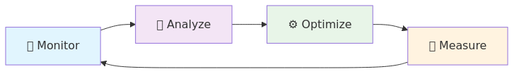
📈 Monitoring and Tuning
🔍 Continuous Improvement
Implement comprehensive monitoring to identify and resolve performance bottlenecks.
📊 Performance Monitoring
📈 Critical Metrics Dashboard
| Metric Category | Key Indicators | Monitoring Tool | Alert Threshold |
|---|---|---|---|
| 🚀 Spark UI Metrics | Stage duration, task skew, shuffle data | Spark History Server | |
| 🔍 Execution Plans | Physical vs. logical plan efficiency | DataFrame explain() | |
| 📊 I/O Performance | Read/write throughput and latency | Azure Monitor |
# 🔍 Query plan analysis for optimization

# Show all execution plan details
df.explain(True)  # Physical, logical, optimized, and code gen plans

# Quick performance check
df.explain("cost")  # Show cost-based optimization details

# Analyze specific operations
df.filter(...).join(...).explain()
📈 Spark UI Key Areas
- Jobs Tab: Overall job duration and failures
- Stages Tab: Task distribution and skew
- Storage Tab: Cached DataFrame efficiency
- Executors Tab: Resource utilization
🔧 Performance Tuning Methodology
| Phase | Action | Success Criteria | Duration |
|---|---|---|---|
| 📊 Baseline | Establish performance metrics | Documented current state | |
| 🔄 Iterative Tuning | One change at a time | 10%+ improvement per iteration | |
| 🔍 Workload Analysis | Pattern-based optimization | Consistent performance |
📋 Tuning Checklist
- 📈 Document baseline metrics
- 🎯 Identify performance bottlenecks
- ⚙️ Apply single optimization
- 📈 Measure impact
- 🔄 Repeat for next optimization
- 📊 Monitor production performance
💰 Cost Optimization
💲 Cost Excellence
Balance performance and cost through intelligent resource management.
📉 Resource Utilization
📈 Auto-Scaling Strategy
| Auto-scaling Component | Configuration | Cost Impact | Performance Impact |
|---|---|---|---|
| 📋 Min Nodes | 2-3 nodes | ||
| 📈 Max Nodes | Based on peak demand | ||
| ⏱️ Idle Timeout | 15-30 minutes |
{
  "autoscale": {
    "minNodeCount": 2,
    "maxNodeCount": 10,
    "enabled": true
  },
  "autoPause": {
    "enabled": true,
    "delayInMinutes": 15
  }
}
📀 Right-Sizing Strategy
| Resource Type | Starting Size | Scaling Trigger | Cost Optimization |
|---|---|---|---|
| 🔥 Spark Pools | Small (4 cores) | CPU > 80% for 10 min | |
| 📊 SQL Pools | DW100c | Query queue > 5 | |
| 🗄️ Storage | Hot tier | Access pattern analysis |
📈 Utilization Monitoring
🗄️ Storage Cost Optimization
🔄 Data Lifecycle Management
| Data Age | Access Pattern | Recommended Tier | Cost Savings |
|---|---|---|---|
| 🆕 < 30 days | Frequent access | Hot tier | |
| 📅 30-90 days | Occasional access | Cool tier | |
| 📜 > 90 days | Rare access | Archive tier |
# 🔄 Implement data lifecycle policies
def configure_lifecycle_policy():
    lifecycle_rules = [
        {
            "name": "MoveTocool",
            "enabled": True,
            "filters": {
                "blobTypes": ["blockBlob"],
                "prefixMatch": ["data/bronze/"]
            },
            "actions": {
                "baseBlob": {
                    "tierToCool": {"daysAfterModificationGreaterThan": 30}
                }
            }
        }
    ]
    return lifecycle_rules
🧩 Vacuum Operations
| Operation | Purpose | Frequency | Storage Savings |
|---|---|---|---|
| 🧩 VACUUM | Remove old data files | Weekly | |
| 📋 Log Cleanup | Clean transaction logs | Monthly |
-- 🧩 Regular vacuum operations
VACUUM sales_data RETAIN 7 DAYS;

-- 📋 Clean up old transaction logs (Delta 2.0+)
VACUUM sales_data RETAIN 30 DAYS DRY RUN; -- Preview cleanup
VACUUM sales_data RETAIN 30 DAYS;         -- Execute cleanup
⚠️ Vacuum Best Practices
- Never vacuum with RETAIN < 7 DAYS in production
- Run VACUUM during low-activity periods
- Consider time travel requirements when setting retention
🎆 Performance Optimization Summary
🚀 Excellence Achieved
Optimizing performance in Azure Synapse Analytics requires a holistic approach covering storage organization, query design, resource configuration, and ongoing monitoring.
🏆 Key Success Metrics
| Performance Area | Target Improvement | Measurement Method |
|---|---|---|
| 🔍 Query Performance | 2-5x faster queries | Query execution time |
| 💰 Cost Optimization | 30-60% cost reduction | Monthly Azure spend |
| 📈 Resource Efficiency | 80%+ utilization | CPU/Memory monitoring |
| 🚀 User Experience | < 10s response time | End-user feedback |
🔄 Continuous Improvement Process
💡 Remember Performance optimization is an iterative process that should be tailored to your specific workload characteristics and business requirements. Start with the highest-impact optimizations and measure results before proceeding.
🔗 Next Steps Ready to implement? Start with our Delta Lake optimization examples for hands-on guidance.